1   Introduction

This application note discusses the use of precomputed directional visibility, along with environment maps, for fast interactive lighting and re-lighting of complex scenes. Both the directional visibility at each point and the illumination from an environment map are represented as spherical harmonics. This makes the computation of the environment illumination of the scene a simple dot product of the two sets of spherical harmonic coefficients, which is fast enough to be interactive.

This functionality is new for PRMan version 16.0.

2   Computing directional visibility

The directional visibility at each shading point in the scene can be computed once and for all using either the ptfilter stand-alone program, or the RenderMan Shading Language occlusion() function.

surface
bake_areas( uniform string filename = "", displaychannels = "" )
{
  normal Nn = normalize(N);
  float a, opacity;

  a = area(P, "dicing"); // micropolygon area
  opacity = 0.333333 * (Os[0] + Os[1] + Os[2]); // average opacity
  a *= opacity; // reduce area if non-opaque

  if (a > 0)
    bake3d(filename, displaychannels, P, Nn, "interpolate", 1, "_area", a);

  Ci = Cs * Os;
  Oi = Os;
}

ptfilter -filter occlusion -shbands 3 dragon_areas.ptc dragon_dirvis3.ptc

3   Computing spherical harmonics for an environment map

The txmake utility program can be used to compute a spherical harmonic representation of an environment map. The environment map can be in lat-long or cube-map format, and the input image format can be any of the many image formats that txmake supports. The spherical harmonic coefficients are simply stored in the output image file itself (in the header or tail of the file, depending on the image format). Currently the output image has to be in OpenEXR or TIFF format.

For example, to compute five spherical harmonic bands (25 coefficients) for the environment map "rosette_hdr.env", and embed them in the lat-long image "rosette.tex", we can call txmake like this:

txmake -envlatl -shbands 5 rosette_hdr.env rosette.tex

(The default value of shbands is 0, which means that no spherical harmonics are computed.) The image type has to be envlatl or envcube.

A shader can then read the environment map's spherical harmonic coefficients using the textureinfo() function:

textureinfo(envmap, "shcoeffs", envmapshcoeffs);

(Alternatively, the spherical harmonic representation of the environment map can also be computed in a DSO. This is less elegant than doing it in txmake, among other reasons because they have to be computed every time the environment map is being used for rendering.)

4   Rendering image-based lighting

At this point we have both directional visibility (at each point) and the environment map represented as spherical harmonic coefficients. Computing the environment illumination at each point can now be done by convolving the the two sets of coefficients. The advantage of the spherical harmonic representation is that convolution is simply done by a dot product of the coefficients, so it is basically just a few multiplies and adds at each shading point. Hence it is very fast!

Here is a shader example that convolves the environment map's spherical harmonic (color) coefficients with the directional visibility's spherical harmonic (float) coefficients.

The environment map's spherical harmonic coefficients are read using textureinfo() and then converted to the built-in data type stdrsl_SphericalHarmonic. Since the environment map is the same for all surface points, the coefficients are only read once per grid. The coefficients can optionally be rotated, corresponding to rotating the environment map.

At each shading point, the directional visibility's spherical harmonic (float) coefficients are read from a point cloud using texture3d(). The coefficients are then converted to the stdrsl_SphericalHarmonic data type and convolved with the environment map coefficients using the built-in function convolve().

#include <stdrsl/SphericalHarmonics.h>

//
// Fast convolution of environment map with precomputed directional
// visibilities.  Lookup directional visibility SH coefficients in
// point cloud and multiply them with SH coefficients for environment
// map.  The sum of the products is the environment map illumination.
//
surface
fastenvillum(string envmap = "", envspace = "", dirvisfile = "";
             float windowingmode = 0)
{
  uniform stdrsl_SphericalHarmonic envmapsh;
  uniform color envmapshcoeffs[]; // varying-length array
  stdrsl_SphericalHarmonic dirvissh;
  float dirvisshcoeffs[]; // varying-length array
  color envcol = 0;
  float ok;

  // Get environment map SH coeffs (same for entire point cloud).
  // The envmapshcoeffs array is automatically resized to fit the
  // number of SH coefficients in the environment map.
  // (Since this is the same for the entire point cloud, this could
  // be done in an init shader.)
  textureinfo(envmap, "shcoeffs", envmapshcoeffs);

  // Construct standard spherical harmonics type from array of coeffs
  envmapsh->createFromArray(envmapshcoeffs);

  // Rotate the SH coeffs if required
  if (envspace != "")
    envmapsh->rotate(envspace);

  // Lookup directional visibility SH coefficients in point cloud.
  // The dirvisshcoeffs array is automatically resized to fit the
  // number of SH coefficients in the point cloud file.
  ok = texture3d(dirvisfile, P, N, "_dirvisshcoeffs", dirvisshcoeffs);

  if (ok != 0) {
    // Construct standard spherical harmonics type from array of coeffs
    dirvissh->createFromArray(dirvisshcoeffs);

    // Convolve directional visibility SH coeffs with env map SH coeffs.
    // The convolution is simply a dot product; the result is a color.
    // If windowing is turned on, heigher bands (higher frequencies) are
    // weighted less, resulting in reduced ringing (smaller oscillations).
    envcol = envmapsh->convolve(dirvissh, windowingmode);
  }

  Ci = envcol * Cs * Os;
  Oi = Os;
}

The image below shows the result of running this shader on a dragon scene:

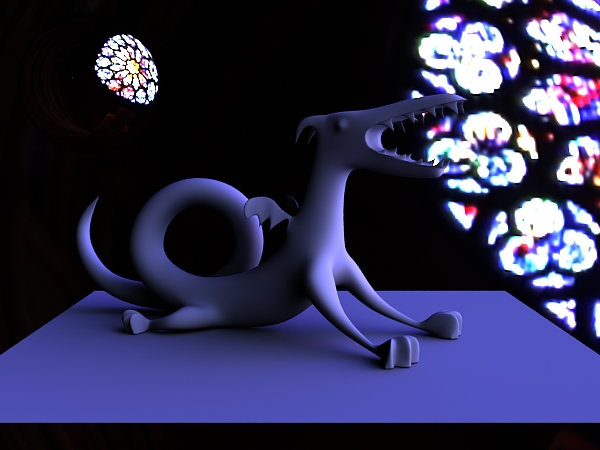
Dragon scene illuminated by the Rosette environment map

Notice how the illumination on the dragon and the soft shadows correspond to the environment map.

There is a sphere in the upper left corner which shows a reflection of the environment map. The background of the image shows part of the same environment map, projected onto a half-sphere behind the rest of the scene.

Rendering this image at 1K resolution on a modern multi-core computer only takes a few seconds. That's fast enough that rotating or changing the environment map (and recomputing its spherical harmonic coeffients) can be done interactively, and the image can be re-rendered many times until the illumination is as desired.

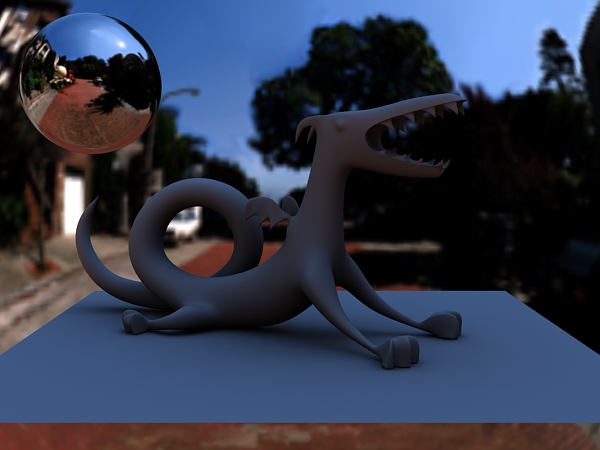
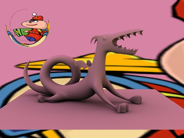
The images below show the same scene illuminated by a few other environment maps:

# Coordinate system for rotating LatLong env map such that top of the
# map image is in the +y axis direction and the center of the map image
# is in the +z axis direction.  In other words: up is up, center is
# straight ahead, and left and right edges are behind.
TransformBegin
  Rotate 90 1 0 0    # rotate 90 degrees around x axis
  Rotate -90 0 1 0   # rotate -90 degrees around y axis
  CoordinateSystem "rotateLatLong"
TransformEnd

5   Computing directional color bleeding

As a step beyond environment illumination, we can also compute a spherical harmonic representation of the directional variation of the indirect illumination at each point.

The first step is to generate a point cloud with area and direct illumination data. The second step is to call ptfilter with the colorbleeding filter to compute the spherical harmonics.

For example, if we want to compute the first five spherical harmonic bands (25 coefficients) for a point cloud of a (directly) illuminated dragon, we can call ptfilter like this:

ptfilter -filter colorbleeding -shbands 5 -sortbleeding 1 dragon_radio.ptc dragon_irrad5.ptc

In addition to the _dirvisshcoeffs[] array, there is also an _incradshcoeffs[] array in the dragon_irrad5.ptc point cloud. The latter is a spherical harmonic representation of the incident indirect illumination at each point. The coefficients can be inspected with ptviewer.

Alternatively, the indirectdiffuse() function can be used to compute the same results. Like occlusion(), the indirectdiffuse() function has a new optional parameter "shbands", and it has two optional output variables: the float dirvisshcoeffs[] array and color incradshcoeffs[] array.

6   Summary

Image-based lighting and relighting is fast enough that it can be used as an interactive technique for designing and fine-tuning environment illumination of complex scenes.

An additional use is for computing the directional variation of indirect illumination.

7   More information

More information about spherical harmonics can be found in the following references:

• Press, Flannery, Teukolsky and Vetterling, Numerical Recipes in C, Cambridge University Press.
• Francois Sillion, Jim Arvo, Steven Westin and Donald Greenberg, "A global illumination solution for general reflectance distributions", Proc. SIGGRAPH 1991, pp. 187-196.
• Ravi Ramamoorthi and Pat Hanrahan, "An efficient representation for irradiance maps", Proc. SIGGRAPH 2001, pp. 497-500.
• Peter-Pike Sloan, "Stupid spherical harmonics tricks", Microsoft tech report, 2008.
• Matt Pharr and Greg Humphreys, Physically Based Rendering: From Theory to Implementation, 2nd edition, Elsevier, 2010.

Another way to compute spherical harmonics for directional visibility -- and a great example of their use for interactive image-based relighting -- is presented in this paper:

• Jacopo Pantaleoni, Luca Fascione, Martin Hill and Timo Aila, "PantaRay: Fast ray-traced occlusion caching of massive scenes", Proc. SIGGRAPH 2010, article 37.